Locating KBAs: An automated workflow for identifying potential Key Biodiversity Areas
The following workflow is designed to facilitate and streamline the scoping analysis for KBA identification by leveraging the free and open access data of GBIF.
The workflow is divided into three main steps:
Select the species in the study area that could potentially trigger KBA criteria.
Identify the sites where the potential trigger species occur in significant numbers.
You may want to add/remove steps or modify the code based on your interests.
Before running the code, I recommend visiting this link and familiarizing yourself with the different KBA criteria and their associated thresholds.
Setup
Load the libraries
library(tidyverse) # To do data wrangling
library(Hmisc) # To use the %nin% binary operator
library(rgbif) # To access records through the GBIF API
library(wellknown) # To handle Well Known Text Objects
library(rredlist) # To access IUCN information
library(ggplot2) # To create graphics
library(ggspatial) # To add north arrows and annotation scales to ggplot maps
library(RCurl) # To compose HTTP requests
library(xml2) # To work with HTML and XML
library(rvest) # To download and manipulate HTML and XML
library(sf) # To work with vector data
library(sp) # To work with vector data
library(DT) # To display tables in the notebook
library(leaflet) # To make interactive maps
library(knitr) # To knit the document
library(foreach) # For parallelization of loops
library(doSNOW) # For parallelization of loops
library(parallel) # For parallelization of loops
library(stringi) # To remove special characters of species common names
library(CoordinateCleaner) # To flag potentially problematic coordinate records
library(countrycode) # For turning country codes into ISO-3 country codes
library(taxadb) # To find species accepted namesDefine initial configuration parameters
# Increase the time allowed to access URLs
curlSetOpt(timeout = 100000)## An object of class "CURLHandle"
## Slot "ref":
## <pointer: 0x0000013444f18600># Disable scientific notation
options(scipen=999)To access GBIF data, you must have an account on the platform. If you do not have one, create it by entering the following link. Additionally, to access IUCN information, you must request an API key here.
Once you have both the account and the API key, you can define new variables to store them. The following are just examples that you can replace with your information.
GBIF_USER <- "pp"
GBIF_PWD <- "pphh"
GBIF_EMAIL <- "pp@gmail.com"
IUCN_REDLIST_KEY = "12345"1. Select potential trigger species
1.1. The first thing we will do is download the occurrence records present in our study area. Save the shapefile of your study area in the data folder. For this example, we will focus the scope analysis on the department of Quindío in Colombia.
# Load shapefile of the study area
st_area <- st_read("data/Quindio.shp", quiet = TRUE)
# Convert shapefile into a Well Known Text object (WKT)
wkt <- wellknown::sf_convert(st_area)You can also set additional conditions for the data you want to download. Since we are going to explore the spatial location of potential trigger species, I will only download records that have coordinates. Also, I will only use records taken recently.
# Download GBIF records
download <- occ_download(
# Records with coordinates
pred("hasCoordinate", TRUE),
# Records taken between 2017 and 2021
pred_gte("year", 2017),
pred_lte("year", 2022),
# Records that fall within the study area
pred_within(wkt),
# Records that fall within Colombia
pred("country", "CO"),
# Format of the resulting file
format = "SIMPLE_CSV",
# GBIF account information
user = GBIF_USER,
pwd = GBIF_PWD,
email = GBIF_EMAIL)After submitting the download request to GBIF, we must wait a few minutes for it to be accepted.
# Check download status
occ_download_meta(download)$status## [1] "SUCCEEDED"Once the request status is successful, we can download the data
# download the data
z <- occ_download_get(download, path = "data/", overwrite = TRUE)# Import data to an R dataset
data <- occ_download_import(z)Now, we will plot the study area and the records downloaded from GBIF, to verify that all the points fall within our polygon of interest.
# Turn dataset into an sf object
data_sf <- st_as_sf(data, coords = c("decimalLongitude", "decimalLatitude"), crs = 4326)
# Plot points and study area
ggplot(data = st_area) +
geom_sf() +
xlab("Longitude") + ylab("Latitude") + # Change x and y labels
geom_sf(color = "black", fill = "grey") + # Change polygon and line color
geom_sf(data=data_sf, color = 'green') + # Add occurrence records
annotation_scale() + # Add an annotation scale
annotation_north_arrow(location='br') + # Add the north arrow to the bottom right
ggtitle("Occurrence records that fall within the study area") # Add title to map 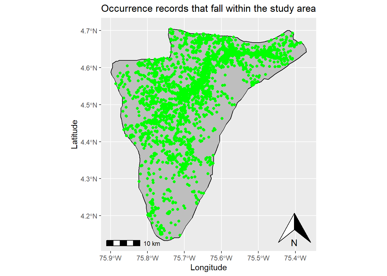
# Remove variable
rm(data_sf)1.2. We will now clean the occurrence dataset because this reduces the probability of including erroneous records and ensures that the data are suitable for the analysis (Gueta & Carmel, 2016).
## [1] "Number of initial records: 244433"# Remove duplicates
data_wDuplicates <- data %>%
# Remove records that have the same combination of the following variables
distinct(decimalLongitude,decimalLatitude,speciesKey,datasetKey,eventDate,individualCount,basisOfRecord, .keep_all = TRUE)
# Remove previous dataset
rm(data)## [1] "Number of records without duplicates: 163983"Records obtained from GBIF may have issues and flags that indicate common quality problems. Therefore, it is important to explore the issues present in our dataset and remove the records that you consider inappropriate for the scoping analysis
# Examine the GBIF issues present in our dataset
data_issues <- str_split(unique(data_wDuplicates$issue), ";") %>%
# Get a list of the issues present in the dataset
unlist() %>% unique()# Obtain the definition of the GBIF issues present in our dataset
GBIF_issues <- gbif_issues() %>%
filter(issue %in% data_issues)
print(paste(GBIF_issues$issue, GBIF_issues$description))## [1] "COORDINATE_ROUNDED Original coordinate modified by rounding to 5 decimals."
## [2] "COUNTRY_DERIVED_FROM_COORDINATES The interpreted country is based on the coordinates, not the verbatim string information."
## [3] "ELEVATION_MIN_MAX_SWAPPED Set if supplied min > max elevation"
## [4] "GEODETIC_DATUM_ASSUMED_WGS84 Indicating that the interpreted coordinates assume they are based on WGS84 datum as the datum was either not indicated or interpretable."
## [5] "MULTIMEDIA_URI_INVALID An invalid uri is given for a multimedia object."
## [6] "TAXON_MATCH_FUZZY Matching to the taxonomic backbone can only be done using a fuzzy, non exact match."
## [7] "TAXON_MATCH_HIGHERRANK Matching to the taxonomic backbone can only be done on a higher rank and not the scientific name."
## [8] "OCCURRENCE_STATUS_INFERRED_FROM_INDIVIDUAL_COUNT Occurrence status was inferred from the individual count value"
## [9] "AMBIGUOUS_COLLECTION The given collection matches with more than 1 GrSciColl collection."
## [10] "INSTITUTION_MATCH_FUZZY The given institution was fuzzily matched to a GrSciColl institution."
## [11] "INSTITUTION_MATCH_NONE The given institution couldn't be matched with any GrSciColl institution."If you want to delete records with specific problems, you can use the following example code. However, for this example, I will not delete any of the records with issues.
data_wIssues <- data_wDuplicates[which(grepl(paste(c("TAXON_MATCH_HIGHERRANK", "INSTITUTION_MATCH_NONE"), collapse = "|"), data_wDuplicates$issue) == FALSE), ]## [1] "Number of presence records after removing issues: 163983"The coordinateCleaner package also provides some tools to flag records with common spatial errors, such as records assigned to the centroid of a country or province, the headquarters of GBIF or other biodiversity institutions. We will use this package to flag suspicious records, but we will not delete any in this example. It is recommended that you further explore flagged records before removing them from the analysis.
# Turn into ISO-3 country codes
data_wDuplicates$countryCode <- countrycode(data_wDuplicates$countryCode, origin = 'iso2c', destination = 'iso3c')
# Identify records with potential spatial errors
data_wDuplicates <- clean_coordinates(x = data_wDuplicates,
lon = "decimalLongitude",
lat = "decimalLatitude",
countries = "countryCode",
species = "species",
tests = c("capitals", "centroids",
"equal","institutions",
"zeros", "countries")) ## Testing coordinate validity## Flagged 0 records.## Testing equal lat/lon## Flagged 0 records.## Testing zero coordinates## Flagged 0 records.## Testing country capitals## Flagged 0 records.## Testing country centroids## Flagged 181 records.## Testing country identity## Flagged 0 records.## Testing biodiversity institutions## Flagged 2719 records.## Flagged 2900 of 163983 records, EQ = 0.02.You can use the following dataset called “flagged_records” to further explore the records with potential issues
# Filter flagged records
flagged_records <- data_wDuplicates %>% filter(.summary == FALSE) %>% droplevels()
# Plot flagged and non-flagged records
ggplot(data = st_area) +
geom_sf() +
xlab("Longitude") + ylab("Latitude") + # Change x and y labels
geom_sf(color = "black", fill = "grey") + # Change polygon and line color
geom_sf(data=(st_as_sf((data_wDuplicates %>% filter(.summary == TRUE) %>% droplevels()), coords = c("decimalLongitude", "decimalLatitude"), crs = 4326)),color = 'green') + # Add occurrence records that were not flagged
geom_sf(data=(st_as_sf(flagged_records, coords = c("decimalLongitude", "decimalLatitude"), crs = 4326)),color = 'red') + #Add flagged records
annotation_scale() + # Add an annotation scale
annotation_north_arrow(location='br') + # Add the north arrow to the bottom right
ggtitle("Flagged occurrence records in red") # Add title to map 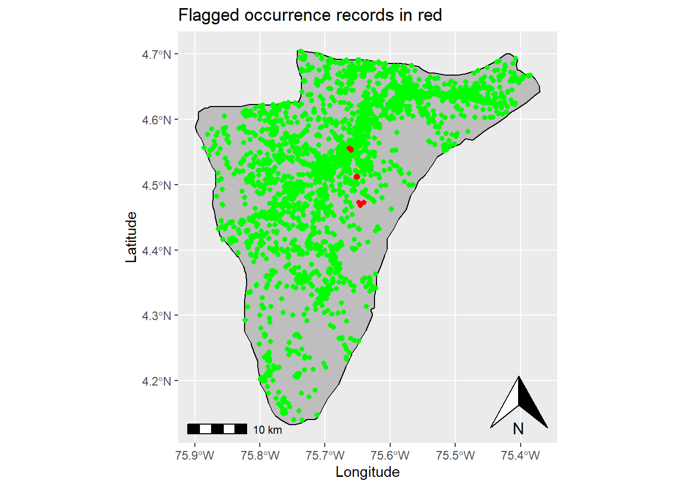
Next, we will remove the records that are not identified at least at the species level, because the thresholds associated with the species-based criteria are designed to be applied at this taxonomic level (KBA Standards and Appeals Committee, 2020).
We will also delete the absence records, as they do not provide information on the species present in the study area.
data_spLevel <- data_wDuplicates %>%
# Select the records where the taxon rank is at least species
filter(taxonRank == "SPECIES" | taxonRank == "SUBSPECIES" | taxonRank == "VARIETY") %>%
# Select presence records
filter(occurrenceStatus == "PRESENT") %>%
# drop levels
droplevels()
# Remove previous dataset
rm(data_wDuplicates)## [1] "Number of records identified at least at the species level: 163645"The taxonomy used for KBA identification should be consistent with the taxonomic backbone of the IUCN Red List, i.e., the Species Information Service, SIS (KBA Committee on Standards and Appeals, 2020). Thus, we will exclude records with unrecognized species names based on the IUCN Red List assessments.
In addition, we will eliminate the records of species introduced (non-native) in our study area since these cannot trigger KBAs (KBA Committee on Standards and Appeals, 2020).
# Create a table with the species names present in the occurrence dataset
list_species <- data_spLevel %>%
# Get unique species names
distinct(species, .keep_all = TRUE) %>%
# Keep species taxonomy
select(kingdom, class, order, family, species) ## [1] "Number of species: 1657"The following chunk is a parallelized loop that uses several of your computer’s cores to speed up the process of finding the species names under the IUCN taxonomic backbone. By default, it uses the total number of cores on your computer minus 2. If you want to change this, modify the variable called “cl”.
# Create a cluster
cl <- makeCluster(detectCores()-2)
# Register the cluster
registerDoSNOW(cl)
# Define the number of iterations
iterations <- length((1:nrow(list_species)))
# Create a progress bar based on the number of iterations
pb <- txtProgressBar(max = iterations, style = 3)
progress <- function(n) setTxtProgressBar(pb, n)
opts <- list(progress = progress)
join1 <- foreach(i = (1:nrow(list_species)),
.combine = rbind,
.options.snow = opts,
.packages = "rredlist") %dopar%
{
species <- list_species$species[i]
# Verify if the species name is a synonym of the IUCN accepted name
x <- rl_synonyms(name = species, key = IUCN_REDLIST_KEY, parse = TRUE)
# If there are no synonyms
if (length(x$result) == 0) {
# then leave the original name
IUCN_name <- x$name[1]
} else {
# otherwise extract the IUCN accepted name
IUCN_name <- x$result$accepted_name[1]
}
# Slow down the loop for 3 seconds as too many frequent calls can temporarily block access to the IUCN API
Sys.sleep(3)
# Use another rredlist function to find out if the name has any information associated with it or if it can't be found
x2 <- rl_occ_country(IUCN_name, key = IUCN_REDLIST_KEY, parse = TRUE)
#If there is no info, it could be because the species name does not have a red list assessment. This could be checked manually.
if ((x2$count) == 0) {
IUCN_name <- "CHECK"
}
# Slow down the loop for 3 seconds as too many frequent calls can temporarily block access to the IUCN API
Sys.sleep(3)
# Retrieve results
results <- data.frame(cbind(species, IUCN_name))
return(results)
}For the names that could not be recognized using the IUCN API, we will search for the accepted name under the Integrated Taxonomic Information System.
# Create a local copy of the Integrated Taxonomic Information System database
taxadb::td_create("itis")
# Create new field to store ITIS accepted name
join1 <- join1 %>% mutate(ITIS_name = NA)
# Retrieve the ITIS accepted name for the species that were not recognized by the IUCN API
for (i in (which(join1$IUCN_name == "CHECK"))){
# Find the accepted species name under the Integrated Taxonomic Information System
join1$ITIS_name[i] <- taxadb::filter_name(join1$species[i]) %>%
mutate(acceptedNameUsage = get_names(acceptedNameUsageID)) %>%
select(acceptedNameUsage) %>% pull() %>% as.character()
# If the name is not found, leave "CHECK"
if (is.na(join1$ITIS_name[i])){
join1$ITIS_name[i] <- "CHECK"
}
}
# Apply loop to the species that were not recognized by the IUCN API
# and where the ITIS accepted name is different from name recorded in the GBIF dataset
# Define the number of iterations
iterations <- length(which(!is.na(join1$ITIS_name) & join1$ITIS_name != "CHECK" & join1$ITIS_name != join1$species))
# Create a progress bar based on the number of iterations
pb <- txtProgressBar(max = iterations, style = 3)
progress <- function(n) setTxtProgressBar(pb, n)
opts <- list(progress = progress)
# Search for IUCN accepted names for those spcies where the ITIS accepted name
# is different from the name recorded in the GBIF dataset
join1.1 <- foreach(i = (which(!is.na(join1$ITIS_name) & join1$ITIS_name != "CHECK" & join1$ITIS_name != join1$species)),
.combine = rbind,
.options.snow = opts,
.packages = "rredlist") %dopar%
{
species <- join1$species[i]
ITIS_name <- join1$ITIS_name[i]
# Verify if the species name is a synonym of the IUCN accepted name
x <- rl_synonyms(name = ITIS_name, key = IUCN_REDLIST_KEY, parse = TRUE)
# If there are no synonyms
if (length(x$result) == 0) {
# then leave the original name
new_IUCN_name <- x$name[1]
} else {
# otherwise extract the IUCN accepted name
new_IUCN_name <- x$result$accepted_name[1]
}
# Slow down the loop for 3 seconds as too many frequent calls can temporarily block access to the IUCN API
Sys.sleep(3)
#Use another rredlist function to find out if the name has any information associated with it or if it can't be found
x2 <- rl_occ_country(new_IUCN_name, key = IUCN_REDLIST_KEY, parse = TRUE)
#If there is no info, it could be because the species name does not have a red list assessment. This could be checked manually.
if ((x2$count) == 0) {
new_IUCN_name <- "CHECK"
}
# Slow down the loop for 3 seconds as too many frequent calls can temporarily block access to the IUCN API
Sys.sleep(3)
# Retrieve results
results <- data.frame(cbind(species, new_IUCN_name))
return(results)
}
# Join results
join1 <- full_join(join1, join1.1, by = "species") %>%
mutate(IUCN_name = case_when(IUCN_name != new_IUCN_name & !is.na(new_IUCN_name) ~ new_IUCN_name,
TRUE ~ IUCN_name)) %>%
select(species, IUCN_name)
# Remove temporary dataset
rm(join1.1)
# Stop cluster
stopCluster(cl)## [1] "Number of species without an IUCN name: 690"## [1] "Number of species with an IUCN name: 967"# Include the IUCN name to the GBIF dataset
data_spLevel <- full_join(data_spLevel, join1, by = "species") %>%
filter(IUCN_name != "CHECK") %>%
droplevels()To identify whether occurrences are native or exotic/introduced to our study area, we will use spatial data associated with global Red List assessments which describe native and alien ranges of species.If you are only considering one species in this scoping exercise, you can download its distribution polygon from its assessment website. For example if you want to download the distribution of the species Zimmerius chrysops, you can do it from this website
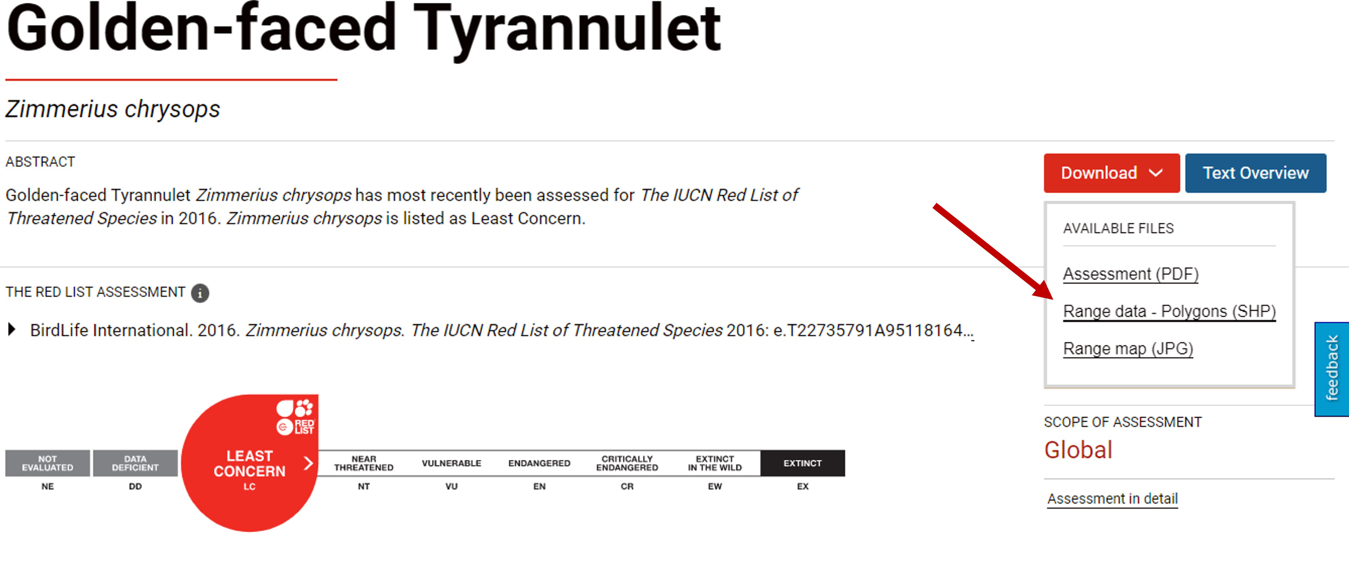
How to download species distributions from their assessment webiste
If you are analyzing several species you can download the distribution polygons for large taxonomic groups from this website. Please note that for bird species you must request a copy of the shapefiles from Birdlife International and this may take several days.
In this example we will focus only on birds and terrestrial mammals.
We will also use the distributions of the global Red List assessments to extract the seasonality of occurrence records. For example, to identify whether the occurrences of migratory species are within the breeding or non-breeding ranges.
Note: Since files containing distributions for large taxonomic groups are very heavy, I recommend clipping them to a smaller extent before uploading them to R to increase performance.
# Load polygons for the different groups
terrestrial_mammals <- st_read("./data/distributions/MAMMALS_TERRESTRIAL_CLIP.shp", quiet = TRUE)
birds <- st_read("./data/distributions/Birdlife_distributions_clip.shp", quiet = TRUE)
# Select origin and seasonal fields
birds <- birds %>% rename(binomial = sci_name) %>% select(binomial, origin, seasonal, citation)
terrestrial_mammals <- terrestrial_mammals %>%
select(colnames(birds))
# Merge everything into the same dataset
distributions <- rbind(terrestrial_mammals, birds)
# Remove non-merged polygons
rm(terrestrial_mammals, birds)
# Remove polygons of species that are not recorded in the study area
distributions <- distributions[which(distributions$binomial %in% data_spLevel$IUCN_name), ]
# Remove occurrences of species that do not have a distribution
data_spLevel <- data_spLevel %>% filter(IUCN_name %in% unique(distributions$binomial)) %>% droplevels()
# Create a table with the resulting species names
list_species <- data_spLevel %>%
# Get unique species names
distinct(IUCN_name, .keep_all = TRUE) %>%
# Keep species taxonomy
select(kingdom, class, order, family, IUCN_name)
# Create a cluster
cl <- makeCluster((detectCores() - 2))
# Register the cluster
registerDoSNOW(cl)
# Define the number of iterations
iterations <- nrow(list_species)
# Create a progress bar based on the number of iterations
pb <- txtProgressBar(max = iterations, style = 3)
progress <- function(n) setTxtProgressBar(pb, n)
opts <- list(progress = progress)
data_native <- foreach(i = 1:iterations,
.combine = rbind,
.options.snow = opts,
.packages = c("dplyr", "sf")) %dopar%
{
# Turn off the s2 processing
sf::sf_use_s2(FALSE)
# Create a spatial dataframe of the species
occurrences <- data_spLevel %>%
dplyr::filter(IUCN_name == list_species$IUCN_name[i]) %>%
droplevels() %>%
sf::st_as_sf(coords = c("decimalLongitude", "decimalLatitude"), crs = 4326)
# Extract the distribution of that species
ranges <- distributions[which(distributions$binomial == list_species$IUCN_name[i]), ]
# Intersect points(records) and distribution
result <- sf::st_intersection(occurrences, ranges) %>%
# Define origin of records
dplyr::mutate(origin = case_when(origin == 1 ~ "Native",
origin == 2 ~ "Reintroduced",
origin == 3 ~ "Introduced",
origin == 4 ~ "Vagrant",
origin == 5 ~ "Origin Uncertain",
origin == 6 ~ "Assisted Colonisation"),
# Define seasonality of records
seasonal = case_when(seasonal == 1 ~ "Resident",
seasonal == 2 ~ "Breeding Season",
seasonal == 3 ~ "Non-breeding Season",
seasonal == 4 ~ "Passage",
seasonal == 5 ~ "Seasonal Occurrence Uncertain")) %>%
# Create coordinates fields
dplyr::mutate(decimalLongitude = sf::st_coordinates(.)[,1],
decimalLatitude = sf::st_coordinates(.)[,2]) %>%
# Turn to non-spatial dataframe
as.data.frame()
# Retrieve result
return(result)
}
# Stop cluster
stopCluster(cl)
# Remove distributions
rm(distributions)
# Remove non-native species
data_native <- data_native %>%
filter(origin == "Native" | origin == "Reintroduced") %>%
droplevels() %>%
select(-c(binomial, geometry))# Free unused R memory
gc() ## used (Mb) gc trigger (Mb) max used (Mb)
## Ncells 5286107 282.4 9927564 530.2 9927564 530.2
## Vcells 31763216 242.4 63307409 483.0 63300187 483.0## [1] "Number of native species: 434"# Plot native records and removed records (Species records that fall outside their respective distributions are removed in the previous step)
ggplot(data = st_area) +
geom_sf() +
xlab("Longitude") + ylab("Latitude") + # Change x and y labels
geom_sf(color = "black", fill = "grey") + # Change polygon and line color
geom_sf(data=(st_as_sf((data_spLevel %>% filter(occurrenceID %nin% data_native$occurrenceID) %>% droplevels()), coords = c("decimalLongitude", "decimalLatitude"), crs = 4326)),color = 'red') + #Add removed records
geom_sf(data=(st_as_sf((data_native), coords = c("decimalLongitude", "decimalLatitude"), crs = 4326)),color = 'green') + # Add occurrence records of native species
annotation_scale() + # Add an annotation scale
annotation_north_arrow(location='br') + # Add the north arrow to the bottom right
ggtitle("Occurrences of native species (removed records in red)") # Add title to map 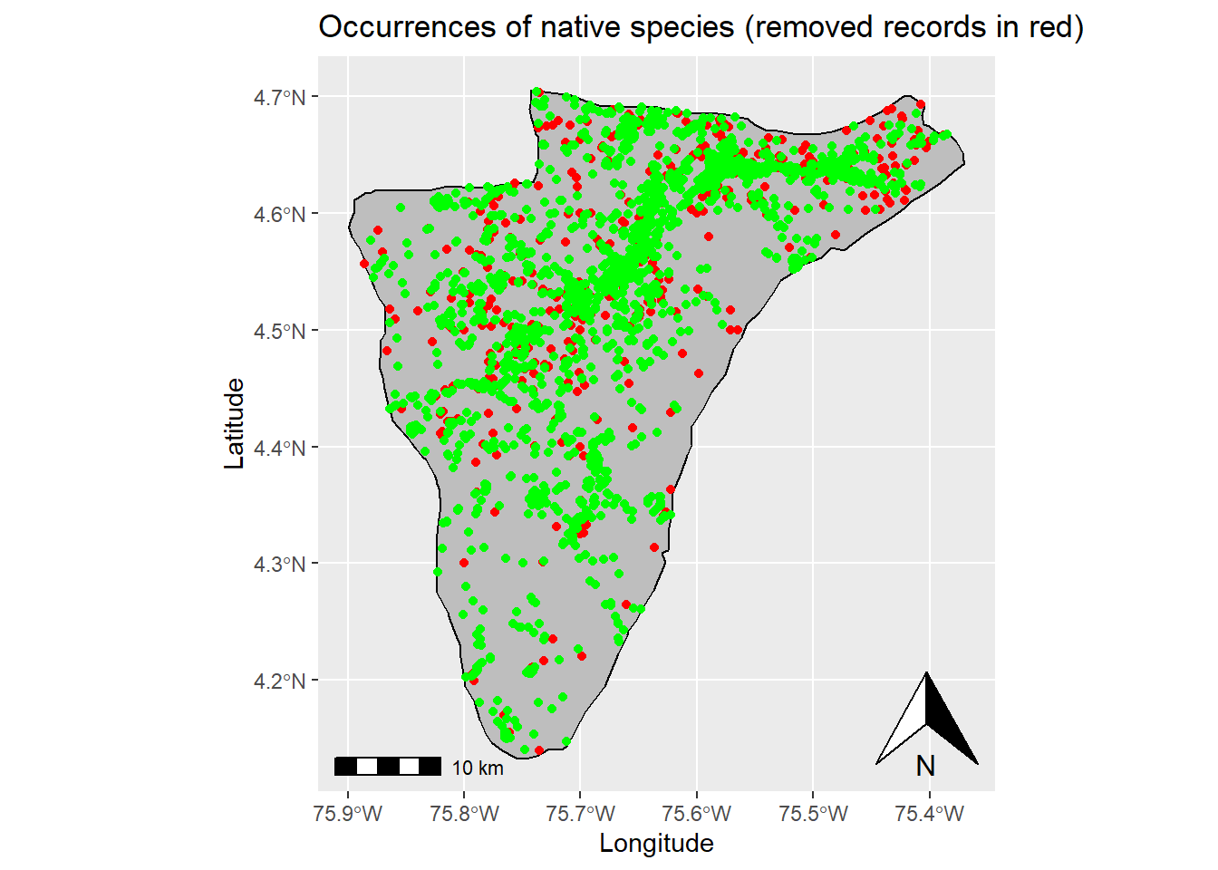
With the resulting table, we can easily identify the species that have a red list assessment and are considered native to our study area.